Google Sheets Tips For SEO

Google Sheets is something we use every day for performing a range of SEO Tasks, from keyword research to tracking progress on projects, and everything in between. It is essentially our bread and butter that we use to bring everything together.

An important part of being efficient on sheets is understanding how you can use the different features and formulas in conjunction with each other to save time. If you are making changes in bulk or entering data manually, more often than not you can save a lot of time using clever use of formulas together.

Knowing how to use Google Sheets in the right way can save you a lot of time in the long run on a wide range of things – and this valuable time could be spent on other SEO tasks. Here is a list of some tips and tricks that you can use to save time on your SEO tasks using Google Sheets.

General Tips

Before we get into the nitty gritty and start looking at formulas, there are a few general tips that might come in handy first. Some of these do similar things to formulas and some of them are basic, but they are still worth familiarising yourself with.

Keyboard Shortcuts

Keyboard shortcuts are simple ways of saving small amounts of time. Although there are plenty of keyboard shortcuts, here are some of the basic and most frequently used ones that everyone should learn in sheets.

Copy (Ctrl/Cmd + C): Copies selected data. Perfect for duplicating keywords, URLs, or SEO stats.

Paste (Ctrl/Cmd + V): Pastes copied content into your current selection. Use it to quickly transfer data like keyword lists across different parts of your spreadsheet.

Cut (Ctrl/Cmd + X): Removes selected data and stores it for pasting elsewhere. Ideal for moving data around your spreadsheet without leaving behind duplicates.

Undo (Ctrl/Cmd + Z): Immediately reverses your last action. Essential for correcting mistakes, such as accidental deletions.

Select All (Ctrl/Cmd + A): Selects all the content in your spreadsheet. Useful for applying formats or functions to entire sheets at once.

Navigate (Ctrl/Cmd + Arrow Keys): Moves the cursor to the edge of data regions. Useful for navigating large sheets of data.

Fill Down (Ctrl/Cmd + Enter): Applies the content of the first selected cell to all cells in the selection. Streamlines the process of filling in repetitive data or formulas.

Paste as Values (Ctrl/Cmd + Shift + V): Allows you to paste the data on your keyboard as static data rather than dynamic data. Useful for converting formulas to hard data.

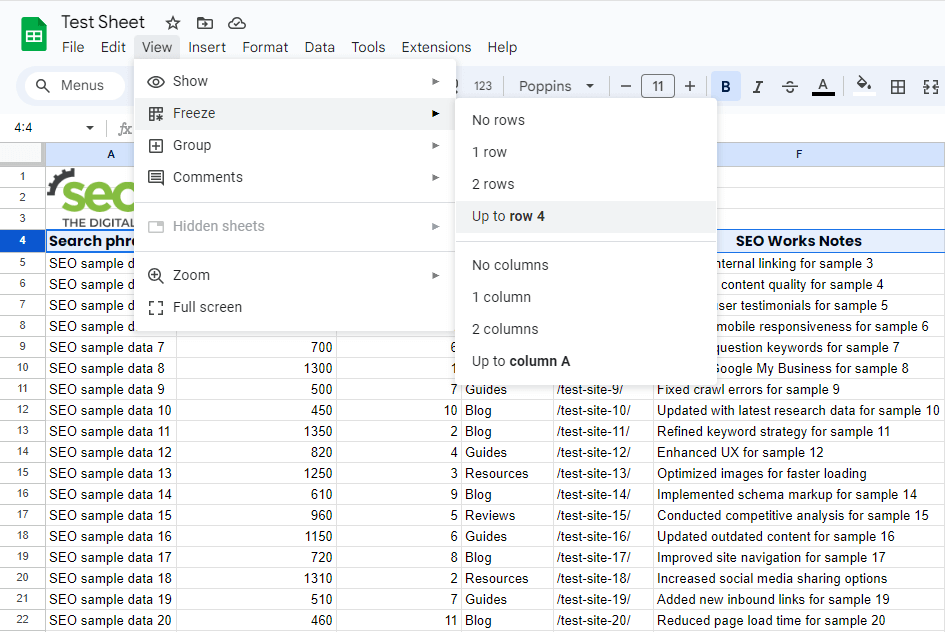
Freeze

Freezing rows or columns lets you keep your headers in place as you scroll through your spreadsheet. This makes it so much easier to navigate through large amounts of data without losing track of what you’re looking at.

How to Access: Select “View” > “Freeze”, then choose the rows or columns you wish to keep in view.

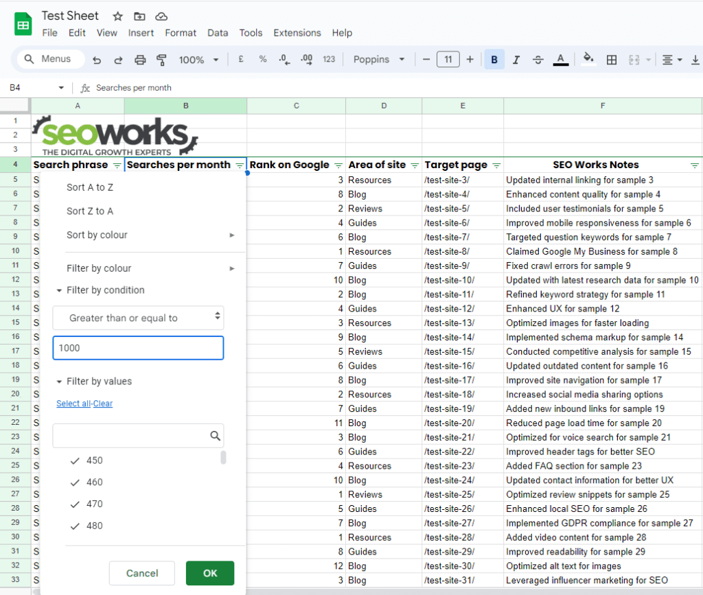
Filters

Filters streamline the process of managing and analysing data by allowing you to display only the rows that meet specific criteria, such as keywords with a search volume above a certain threshold or containing certain phrases.

These are extremely useful for finding something specific, particularly when cross-referenced against each other. You can also copy and paste the data as values into another sheet if you want to extract the data and examine it further.

How to Access: Click “Data” > “Create a filter” to apply filters to your data columns.

Tip: If your data is in a specific order that you would like to keep it in, playing with filters can often result in the order of the data being changed. It is useful to add an additional column with rows numbered from 1, 2, 3 and so on to make sure I can easily restore the original order of my data if you need to.

Tip: This can be used in conjunction with various other formulas if you want to use custom filters.

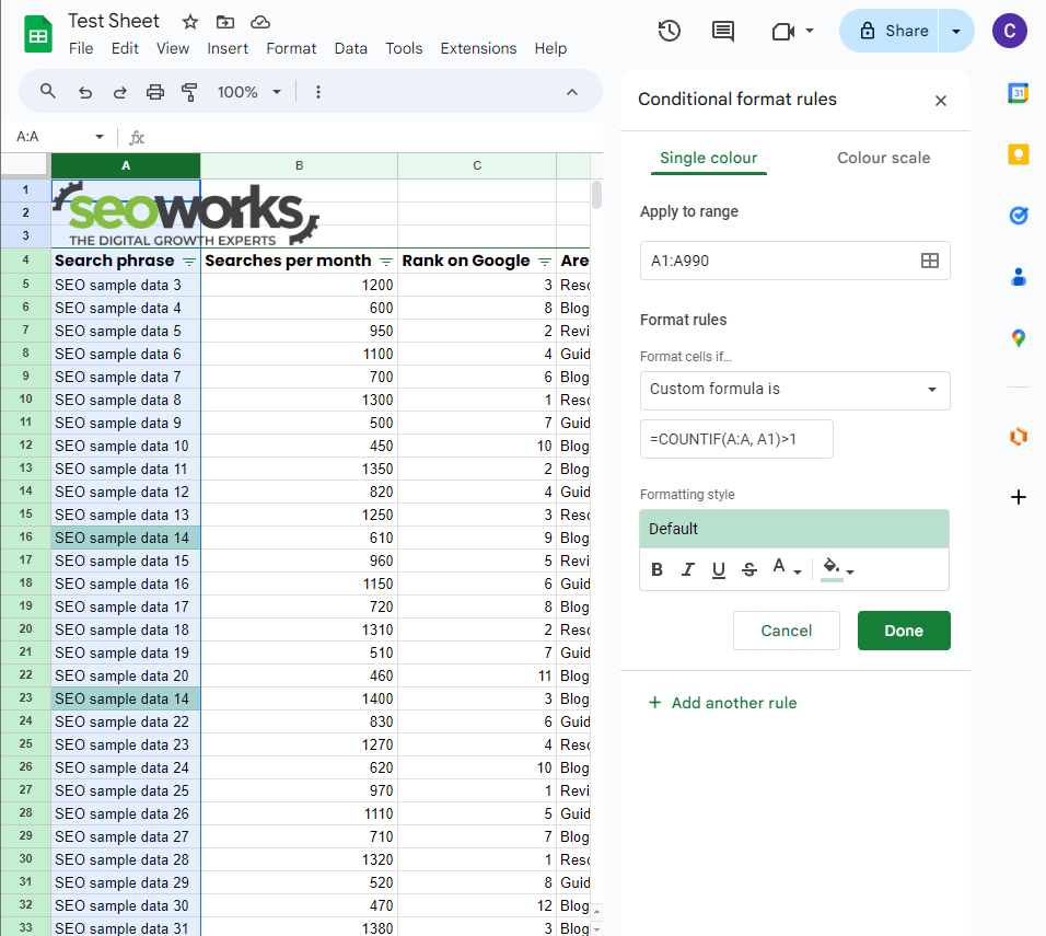
Conditional Formatting

Conditional Formatting highlights information automatically depending on certain criteria. For example, keywords with high search volume or URLs containing specific phrases. It is also useful for highlighting duplicate data if you are working within a large data set before you delete it. You can do this using a COUNTIF formula.

For example, =COUNTIF(A:A, A1)>1 as a custom formula would highlight all duplicate data in column A.

How to Access: Go to “Format” > “Conditional formatting” and set your criteria for formatting.

Tip: This can be used in conjunction with various other formulas if you want to use custom conditional formatting.

Remove Duplicates

Removing duplicates allows you to quickly get rid of duplicate data in a sheet. If you are working with a large dataset it may be better to use conditional formatting and a COUNTIF formula to highlight the data first before deleting it, as some of the corresponding data in other cells may be useful.

However, if you have a smaller data set and you want to quickly get rid of the data then this is useful.

How to Access: Go to “Data” > “Data clean-up” > “Remove duplicates”

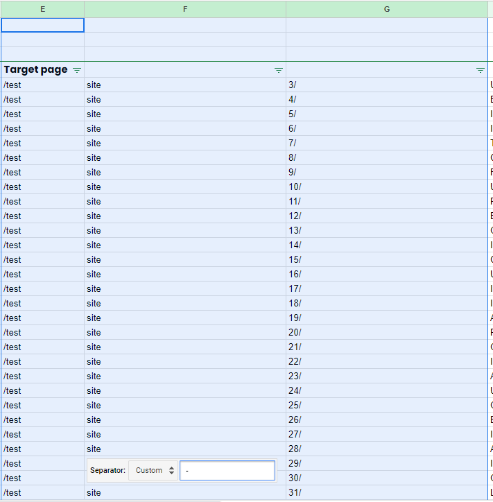
Text To Columns

Text to Columns is a powerful feature for quickly splitting a list of keywords or URLs in a single cell into separate columns based on a specified delimiter. It’s especially useful for organising and restructuring data that it is one cell. It works in a similar way to the SPLIT command.

A delimiter is a designated character that separates data, most commonly a comma but it can be any specific character.

How to Access: Highlight the cell(s), then select “Data” > “Split text to columns” and choose your delimiter.

Tip: You can use this in conjunction with the SUBSTITUTE formula to create delimiters in cells and then break them down easily into multiple cells using this tool.

Tip: Make sure you have plenty of space available as any cells to the right of the data you are splitting may get overwritten. It is always a good idea to add a few extra columns to avoid this and then you can get rid of the blank ones later.

Paste As Values

Using “Paste as Values” allows you to convert dynamic formula results into static text, which is extremely useful when you need to manipulate the results of a formula even more. This feature ensures that your calculated metrics remain constant, even if the source data changes.

How to Access: After copying the desired cells, right-click where you want to paste and choose “Paste special” > “Paste values only”. You can also use the shortcut Ctrl + Shift + V.

Tip: This is something that can be used in conjunction with many of the other features on this list if you are performing multiple formulas to one specific data set.

Formulas

There are over 500 formulas and counting in Google Sheets – some of them are simple and some of them are incredibly complex. Although there are plenty more to learn that aren’t included on our list, here are some of the best ones to know if you are working on SEO tasks.

Formulas Useful For Creating Content and URLs

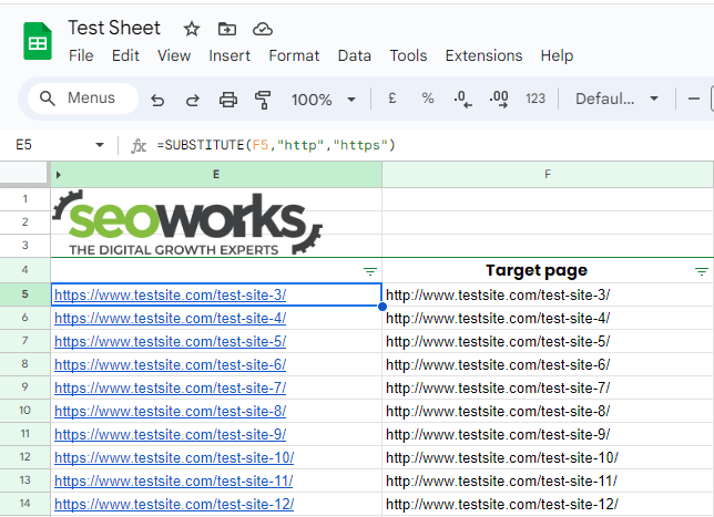
SUBSTITUTE

The SUBSTITUTE function is great for changing large amounts of content in one go, such as bulk updating URLs or tweaking keywords en masse. It searches for a specified substring within a text string and replaces it with another substring.

Syntax: =SUBSTITUTE(text_to_search, search_for, replace_with, [occurrence_number])

text_to_search: The text you want to search through.
search_for: The text you want to find.
replace_with: The text you want to replace the found text with.
[occurrence_number]: (Optional) If specified, only the nth occurrence of the text will be replaced.

Example: If transitioning a website to HTTPS, you might need to update all URLs in column F from http to https. The formula =SUBSTITUTE(F5, “http”, “https”) would quickly make these changes, ensuring that all links reflect the secure protocol.

Tip: This can be embedded into the CONCATENATE function, allowing you to bulk-create URLs from product names or keywords

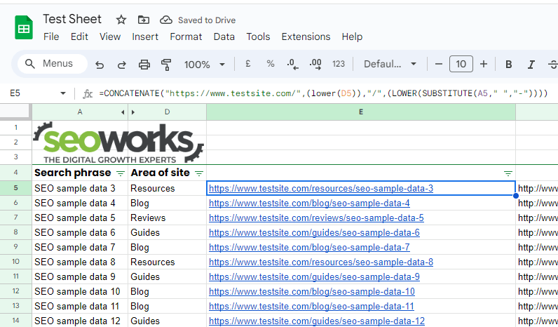
CONCATENATE

CONCATENATE merges multiple text strings into one, making it useful for creating URLs, meta titles, meta descriptions, and more. By combining keywords, slugs, and other necessary elements, you can automate the creation of structured URLs or title tags, ensuring they’re optimised for both users and search engines.

Syntax: =CONCATENATE(text1, [text2, …])

text1, [text2, …]: The text items you want to join together. You can add as many text strings as you need, separated by commas.

Example: To create a URL for a page with the data in cells A5 and D5, you could use =CONCATENATE(“https://www.testsite.com/”,(lower(D5)),”/”,(LOWER(SUBSTITUTE(A5,” “,”-“)))) to create a URL slug from the title and area of the page.

Tip: This can be used with a wide range of other formulas to create a range of different types of content within a specific format.

LEN

The LEN function counts the number of characters in a string. Using LEN, you can make sure your titles and descriptions fit within their character limits.

Syntax: =LEN(text)

text: The text string whose length you want to find. The length includes all characters, including spaces.

Example: To audit meta descriptions for the optimal length, use =LEN(C1) to identify descriptions that exceed the recommended 160 characters, allowing you to revise them for better SERP performance.

Tip: If you want to create meta descriptions or titles in bulk, you can nest an IF statement within a CONCATENATE command to exclude certain strings of text or data if it is already above the character limit.

RIGHT, LEFT, MID

RIGHT and LEFT extract a specific number of characters from a text string, starting from the right or left respectively. These can be important if you want to extract a specific part of a URL in bulk.

Syntax for LEFT: =LEFT(text, [number_of_characters])

text: The text string from which you want to extract characters.
[number_of_characters]: (Optional) The number of characters to extract from the left side of the text. If omitted, it defaults to 1.

Syntax for RIGHT: =RIGHT(text, [number_of_characters])

Similar to LEFT, but extracts characters from the end of the text string.

Example: To extract the year from a URL like “https://example.com/2024/seo-trends” in cell A1, use =LEFT(RIGHT(A1, 9), 4) to get “2024”, which can be useful for categorising content by year.

LEFT, RIGHT, and MID functions are for extracting specific segments from text strings, such as parts of a URL. This allows you to extract a specific number of characters from either the start (LEFT), the end (RIGHT), or any specified part (MID) of the text string.

Syntax for LEFT and RIGHT: =LEFT(text, [number_of_characters])

text: The text string from which you want to extract characters.
[number_of_characters]: (Optional) The number of characters to extract from the left side of the text. If omitted, it defaults to extracting just the first character.

Syntax for MID: =MID(text, start_num, num_chars)

text: The text string from which to extract characters.
start_num: The position of the first character you want to extract.
num_chars: The number of characters to extract.

Tip: Use these functions in conjunction with other commands to extract specific segments of text based on certain characters or delimiters.

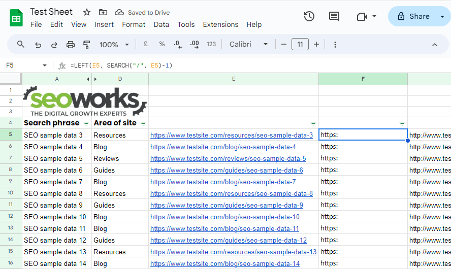
SEARCH

SEARCH finds the position of a text string within another text string. This can be used in conjunction with a range of different formulas to restructure data and pull a specific part of a cell into another cell.

Syntax: =SEARCH(find_text, within_text, [position])

find_text: The text you’re searching for.
within_text: The text within which the search is performed.
[position]: (Optional) The position in the text at which to start the search. If omitted, the search starts at the beginning.

Example: If you have a URL in cell E5, the formula =LEFT(E5, SEARCH(“/”, E5)-1) extracts the URL prefix before the first colon.

Formulas For Cleaning Data

TRIM

The TRIM function is for removing unnecessary spaces from text, whether they occur at the beginning, end, or within the string. This is useful for cleaning any messy data and getting rid of empty spaces caused by human error or formatting issues.

Syntax: =TRIM(text)

text: The string from which you want to remove extra spaces, leaving only single spaces between words and no space at the start or end.

Example: To clean up a list of keywords in cell A1, =TRIM(A1) ensures that each keyword is consistently formatted without leading, trailing, or any hidden spaces.

UPPER, LOWER, PROPER

Capitalisation inconsistencies can skew data analysis and reporting. UPPER, LOWER, and PROPER functions convert text to uppercase, lowercase, or proper case (first letter of each word capitalised), respectively. This can also help avoid duplications based on case differences.

Syntax for UPPER: =UPPER(text)

text: The text you want to convert to uppercase.

Syntax for LOWER: =LOWER(text)

text: The text you want to convert to lowercase.

Syntax for PROPER: =PROPER(text)

text: The text you want to convert to title case (first letter of each word capitalised).

Example: If you have some keywords in cell A1 with rogue capital letters due to human error, =LOWER(A1) would make them lowercase.

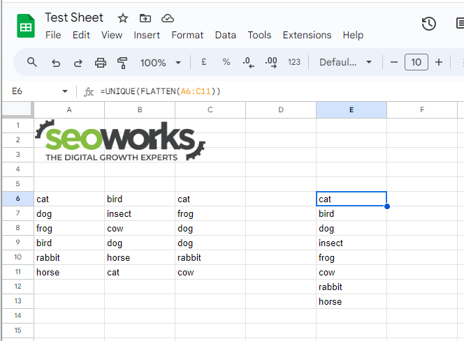
FLATTEN

FLATTEN pulls a range of values across rows and columns and flattens them into a single column, displaying all the data in subsequent cells underneath the formula. This is very useful for cleaning data.

Syntax: =FLATTEN(range)

range: The range of cells you want to convert into a single column

Example: When dealing with data spread across multiple columns, such as keyword lists from different campaigns, =FLATTEN(A1:C10) would consolidate them into a single column starting from where the formula is and all subsequent cells below for the range A1:C10.

Tip: Combine FLATTEN with UNIQUE to consolidate and de-duplicate data at the same time.

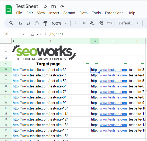
SPLIT

The SPLIT function divides text around a specified character or delimiter, turning a single text string into separate elements. This is particularly useful for parsing complex strings like URLs or long-tail keywords. This works in a similar way to the Split To Columns feature.

Syntax: =SPLIT(text, delimiter, [split_by_each], [remove_empty_text])

text: The string you want to divide.
delimiter: The character or sequence of characters at which you want to split the text.
[split_by_each]: (Optional) TRUE or FALSE to split by each character in the delimiter.
[remove_empty_text]: (Optional) TRUE or FALSE to remove empty text fragments generated by the split.

Example: To analyse the structure of URLs, =SPLIT(F5, “/”) can separate the protocol, domain, and path into individual components.

UNIQUE

UNIQUE is another tool for identifying duplicate data within a dataset. Although conditional formatting with a custom formula may be better for visually identifying which data you want to keep, UNIQUE can be used in conjunction with other commands.

Syntax: =UNIQUE(array_or_range)

array_or_range: The range or array from which you want to extract unique values.

Example: To refine a keyword list, =UNIQUE(A:A) filters out duplicate entries in column A and shows you all the unique cells.

Tip: You can use UNIQUE in conjunction with FLATTEN to de-duplicate data that is spread across multiple columns or sheets.

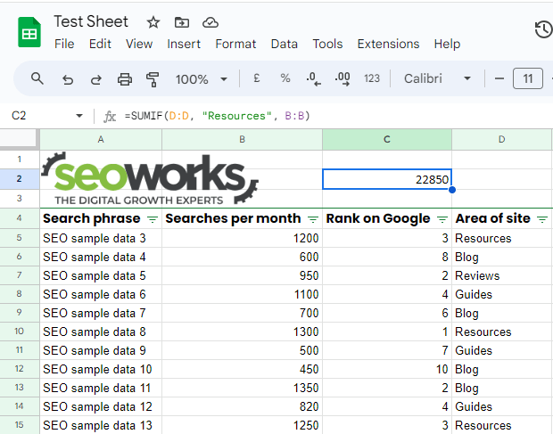
SUMIF

SUMIF calculates values based on a specified condition, allowing you to save time analysing your data, such as calculating total search volumes for a group of keywords.

Syntax: =SUMIF(range, criterion, [sum_range])

range: The range of cells that you’re evaluating against the criterion.
criterion: The condition that determines which cells to sum.
[sum_range]: (Optional) The range from which to sum, different from the range to evaluate.

Example: If column D labels the area of the site, and column B lists searches for month for each keyword, =SUMIF(D:D, “Resources”, B:B) totals the keyword volume for all keywords in the resources area of the site.

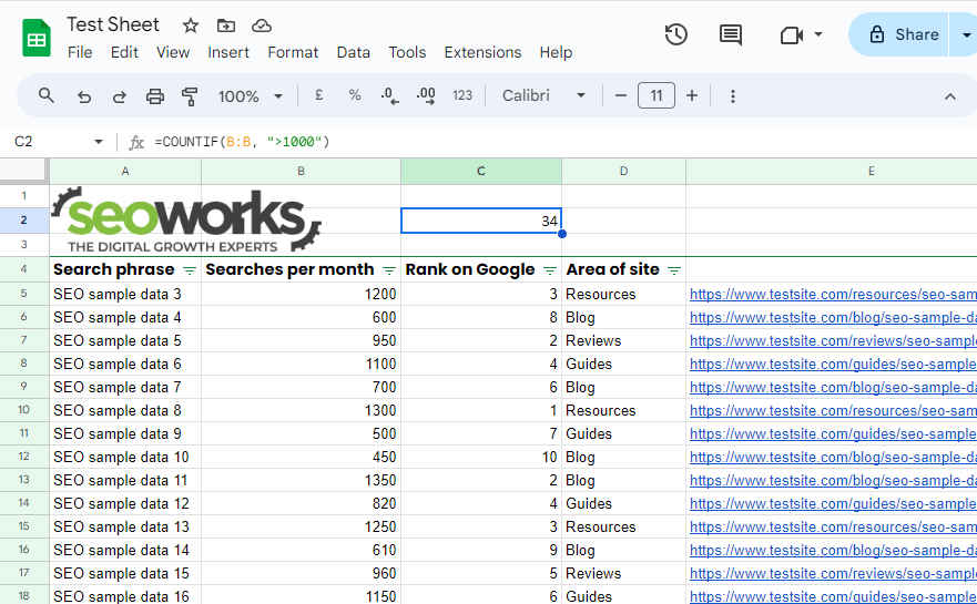
COUNTIF

Similar to SUMIF, COUNTIF counts the number of cells that meet a certain condition. For example, this would be useful if you wanted to check how many keywords you had that had a certain word in, or have a certain search volume.

Syntax: =COUNTIF(range, criterion)

range: The range of cells you’re counting.
criterion: The condition that determines which cells to count.

Example: If column B contains search volumes, =COUNTIF(B:B, “>1000”) counts how many keywords have a search volume over 1000.

COUNTA

This formula works in the same way as COUNTIF, however it shows cells how many cells are not empty. This is good if you have a list of keywords split into different areas of a column and want to check how many are populated.

Syntax: =COUNTA(range)

range: The range of cells you’re counting.

Example: If column A contains only keywords, =COUNTA(A:A) counts how many cells in the column have been populated allowing you to see how many keywords there are.

Formulas Useful For Importing Data

VLOOKUP

VLOOKUP is a very powerful tool for pulling data from different sources. It searches for a value in the first column of a range and returns a value in the same row from a specified column. This is extremely useful in SEO for matching keywords to specific metrics like search volumes or rankings from separate sheets.

Syntax: =VLOOKUP(search_key, range, index, [is_sorted])

search_key: The value you’re looking for in the first column of the range.
range: The range of cells containing the data.
index: The column number in the range containing the return value. For example ‘3’ in this would pull the third column along in your designated range.
[is_sorted]: (Optional) TRUE if the first column in the range is sorted, FALSE for an exact match. For most instances, you would want to use FALSE.

Example: If column A has a keyword in and you have your secondary keywords elsewhere, =VLOOKUP(A6,$H$5:$I$22,2,false) would retrieve the secondary keywords for your primary search phrase from the data range in the screenshot.

Tip: You can use IFERROR with VLOOKUP to handle instances where the lookup value is not found, which will leave your data nice and clean.

Tip: If you are using this formula across multiple cells and your dataset is staying in the same place remember to lock the range of your data by putting a ‘$’ in between the cell letter and cell number. This will prevent your data set from automatically changing if you drag your formula into other cells.

Tip: There is also a ‘HLOOKUP’ command that works in the same way as VLOOKUP which you can use to populate cells horizontally rather than vertically.

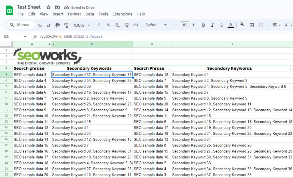
Please note: Usually the data set you are pulling from would be on a different sheet, but in this instance, it is in the same to fit it all in one screenshot.

IMPORTRANGE

IMPORTRANGE imports data from one Google Sheets document to another, which is important if you have data split across different documents. This ensures that all relevant data can be accessed and analysed in a single location with all of the different sheets in sync.

Syntax: =IMPORTRANGE(spreadsheet_url, range_string)

spreadsheet_url: The URL of the spreadsheet from which to import data.
range_string: The range of cells to import, formatted as “sheet_name!range”.

Example: If you need to import a keyword list from another sheet, =IMPORTRANGE(“spreadsheetURL”, “keywords!A:B”) brings in data from “A:B” range of the “keywords” sheet.

IMPORTXML

IMPORTXML is a really useful function for pulling content from a website such as meta titles, meta descriptions, H1 tags, canonical tags, and more. This can save you a lot of time and lets you gather this data in bulk for a range of different pages at once.

Syntax: =IMPORTXML(URL, XPath_query)

URL: The webpage URL from which to import data.
XPath_query: The XPath query that specifies the data or element to be extracted.

There is a wide range of different XPath queries you can use, but here are the most commonly used ones for SEO.

Examples:

XPath for Title Tag: //title

Example: =IMPORTXML(“https://www.seoworks.co.uk”, “//title”) retrieves the title tag of the page.

XPath for Meta Description: //meta[@name=’description’]/@content

Example: =IMPORTXML(“https://www.seoworks.co.uk”, “//meta[@name=’description’]/@content”) retrieves the meta description of the page.

XPath for Canonical Tag: //link[@rel=’canonical’]/@href

Example: =IMPORTXML(“https://www.seoworks.co.uk”, “//link[@rel=’canonical’]/@href”) retrieves the canonical URL for the page.

XPath for H1 Heading: //h1

Example: =IMPORTXML(“https://www.seoworks.co.uk”, “//h1”) retrieves the H1 tags from the page.

Tip: Make sure you press ‘Allow access’ on sheets in order to let Google Sheets pull the data through from an external source – otherwise you may get an error.

Tip: If a page has multiple H1 tags, then these can often spill onto cells below which can sometimes get messy. If you are having trouble with this, there are plenty of free tools available online that will allow you to bulk export H1 tags that you can then work into your sheet.

Other Useful Formulas

ARRAYFORMULA

ARRAYFORMULA allows you to apply a formula to an entire column or range without having to copy the formula down each row. This is incredibly powerful for SEO tasks that involve large datasets, enabling bulk operations like data transformation, extraction, or analysis.

Syntax: =ARRAYFORMULA(array_formula)

array_formula: The formula to apply over an array or range. Allows you to execute multiple calculations on one or more items in a range of cells and display multiple results.

Example: To apply LEN to every Meta Description in a column to check their lengths, =ARRAYFORMULA(LEN(B6:B12)) automates the process, providing immediate insights into potential SEO issues related to URL length.

Advanced Use: Combine ARRAYFORMULA with other functions like VLOOKUP, or IF statements to perform complex data operations on large datasets seamlessly.

GOOGLETRANSLATE

GOOGLETRANSLATE translates text from one language to another, which can be useful for working on international SEO campaigns.

Syntax: =GOOGLETRANSLATE(text, [source_language], [target_language])

text: The string of text to translate.
[source_language]: (Optional) The two-letter language code of the source text. If not set, Google Sheets will attempt to auto-detect the language.
[target_language]: The two-letter language code of the language you want to translate the text into.

Example: If cell A1 says “Hello World” in English, =GOOGLETRANSLATE(A1, “en”, “es”) translates it to “Hola Mundo” in Spanish.

DETECTLANGUAGE

DETECTLANGUAGE identifies the language used in a given text. This can be useful for analysing and sorting through keywords on projects that have global rankings in different languages.

Syntax: =DETECTLANGUAGE(text)

text: The text string whose language you want to identify.

Example: If cell A1 contains “Bonjour”, =DETECTLANGUAGE(A1) detects it’s in French, outputting “fr”.

IFERROR

IFERROR takes care of errors in formulas which makes your data much cleaner.

Syntax: =IFERROR(value, [value_if_error])

value: The formula or expression being evaluated.
[value_if_error]: (Optional) The value to return if the formula evaluates to an error. If not specified, a blank cell is returned.

Example: If a VLOOKUP in cell A1 might cause an error, =IFERROR(VLOOKUP(A1, B:C, 2, FALSE), “Not Found”) shows “Not Found” instead of an error on sheets.

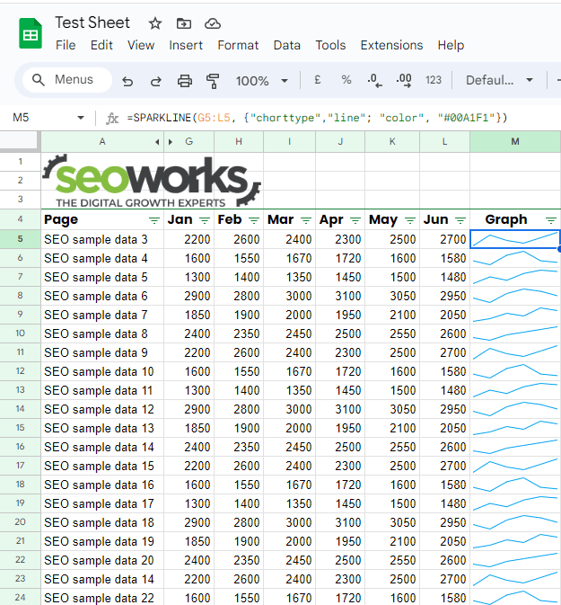
SPARKLINE

SPARKLINE is useful for creating graphs within cells, allowing you to have a visual reference of your data set.

Syntax: =SPARKLINE(data, [options])

data: The range of cells containing the data you want to plot in the sparkline chart.
[options]: (Optional) A set of options to customise the sparkline, specified as a key-value pair in curly braces {}. Common options include “charttype” (which can be “line”, “bar”, “column”, or “winloss”) and “colour”.

Example: If cells G5:L5 contain the monthly search volumes for a specific keyword, =SPARKLINE(G5:L5, {“charttype”,”line”; “color”, “#00A1F1”}) creates a column sparkline chart in a cell, visually displaying the search volume trends with each line coloured in light blue.

Tip: Combine SPARKLINE with IFERROR to make sure if some data points are missing or cause errors, your spreadsheet remains clean and the sparkline chart is displayed without interruption.

Tip: There is a long list of different optional commands you can use to customise your sparkline graphs, but here are some basic ones worth remembering:

charttype: Defines the type of sparkline (options include “line”, “bar”, “column”, “winloss”).
colour: Sets the colour of the chart (accepts named colours or hexadecimal codes).
linewidth: Specifies the thickness of the line in a line chart.
min: Sets the minimum value for the y-axis.
max: Sets the maximum value for the y-axis.

Using ChatGPT to Help With Sheets

Finally, ChatGPT is an excellent tool for creating formulas on sheets. Whilst it is very useful to know commands by heart, if you have a complex task and you are struggling to get the formula down asking ChatGPT can be a good idea.

Although it may not always be correct, most of the time it is. Just make sure you clearly explain exactly what it is you want to do and break it down into small steps. It also helps if you reference the cells (or ranges of cells) you want to work with and more often than not it will be able to output you a command that will work.

Despite this, it is still useful for learning the commands on our list in case something goes wrong on your sheet and you need to correct it, and just to save time in general. Going back to ChatGPT every time you want to add a new formula isn’t the most effective time-saving solution, which is what this guide is all about.

Conclusion

Whilst there are many Google Sheets formulas you can use, it can be very difficult to remember them all. There may be some formulas that you only need to use every once in a while so make sure you bookmark any useful resources (hopefully this blog!) so you can come back to them at a later date.

You don’t need to know every single formula in sheets to save time – the most important thing is having a fundamental understanding of how sheets works, and how the formulas can be integrated together.

Once you have an idea of this you will have a much better idea of areas in which you can save time and ways in which you can manipulate the data to solve complex problems.

If you are interested in learning more about our SEO services, get in touch with our friendly expert team for a chat.

Curtis Halligan

Curtis is a Senior SEO Account Executive with a background in digital marketing & ecommerce.